
1. Introduction
RoboCup Soccer is an international world championship that started in 1997. The event is part of the International Joint Conference on Artificial Intelligence (IJCAI) and set an ambitious target to:
“Foster Artificial Intelligence (AI) and robotics research so that by 2050 a team of autonomous humanoid robots can be built that will be able to win against the human soccer world champion.”
Being multi-agent domain soccer is an interesting as well as challenging domain where agents have to collaborate and cooperate with their team-mates and deal with opponent agents in real-time. It is obvious to note that robotic soccer presents opportunities for application of various specialized areas that include Computer Vision, Robotic Locomotion, real-time Localization, Machine Learning, Algorithmic Optimization, etc. other than the ones that branch out from electronic and mechanical engineering. Various leagues had been setup so that individuals can concentrate on certain aspects of these research areas.
To further help the researchers, simulation leagues were introduced thereby not requiring the research groups to depend on expensive robotic equipment or worry about the engineering aspects. 2D Simulation League was one of the first leagues in RoboCup. Rules have been evolving but in general, two teams of 11 agents compete in a virtual soccer match in real-time. There is a simulation server that receives action commands from the agents and returns a resultant game state to them. The simulation server also controls the game play and provides an automated refereeing of the game. The responses from the server are egocentric – meaning that the positions of objects are sent to agents as distances and directions with respect to the agent itself, this lets the agents to simulate the visual sense of the world and enable the researchers to work their way through to create a real representation of the world model on their own. The server also facilitate aural communication between the agents by providing controlled intervals for each agent to ‘speak’ that can be ‘heard’ by nearby agents. This communication enables the agents to collaborate.
3D Simulation League is a natural extension of the 2D League where the visual information is in 3-dimensions (r, θ, φ). This adds real world complexity for the agents as they now have to handle the height dimension as well. The 3D Simulation League also presents a lot of challenges in terms of locomotion as the agents now can fall to the ground as a result of trying a maneuver that might not be possible by a humanoid robot in a physical world.
The focus of this research is on effective strategies for soccer game play. There is significant research already done in this particular field for 2D Simulation League. It is discussed in detail in Section 3.
2. Key Concepts
During the process of conducting the research, a few theoretical concepts were studied. Below is a quick introduction to these concepts with links to further study.
2.1 Search Algorithms
One of the key areas of implementing strategies in RoboCup is figuring out the optimal path an agent must take. This problem area has been researched under the umbrella term of ‘Path Planning’. Most of the techniques first model the scenario as a graph and then use know graph traversal algorithms to find the optimal path. ‘Optimal’ is a very subjective term in path planning context, it does not necessarily mean the shortest path. Following sections briefly introduce some of the standard graph searching algorithms.
2.1.1 A* Algorithm
A* uses a best-first search approach and finds the most cost-effective path. It was first described by Peter Hart, Nils Nilsson and Bertram Raphael in 1968 [1]. A* is an extension of Edsger Dijkstra’s algorithm published in 1959 [2].
The algorithm uses a two part heuristic function to determine in what sequence a graph is to be traversed. The heuristic function considers:
- The cost from the start node till the current node.
- Estimate of the distance to the goal node.
The constraint for using this function is that the estimate part must be an ‘admissible heuristic’. An admissible heuristic is the one that does not overestimate the distance to the goal node.
The pseudocode for the algorithm is presented at [3] and reproduced below:
function A*(start,goal)
     closedset := the empty set    // The set of nodes already evaluated.
     openset := {start}    // The set of tentative nodes to be evaluated, initially containing the start node
     came_from := the empty map    // The map of navigated nodes.

     g_score[start] := 0    // Cost from start along best known path.
     // Estimated total cost from start to goal through y.
     f_score[start] := g_score[start] + heuristic_cost_estimate(start, goal)

     while openset is not empty
         current := the node in openset having the lowest f_score[] value
         if current = goal
             return reconstruct_path(came_from, goal)

         remove current from openset
         add current to closedset
         for each neighbor in neighbor_nodes(current)
             if neighbor in closedset
                 continue
             tentative_g_score := g_score[current] + dist_between(current,neighbor)

             if neighbor not in openset or tentative_g_score < g_score[neighbor]
                 add neighbor to openset
                 came_from[neighbor] := current
                 g_score[neighbor] := tentative_g_score
                 f_score[neighbor] := g_score[neighbor] + heuristic_cost_estimate(neighbor, goal)

     return failure

function reconstruct_path(came_from, current_node)
     if came_from[current_node] is set
         p := reconstruct_path(came_from, came_from[current_node])
         return (p + current_node)
     else
         return current_node
2.1.2 D* Algorithm
D* is a family of algorithms:
- The informed incremental D* [4].
- The focused D* [5].
- The incremental heuristic search algorithm that builds on LPA* called D* Lite [6].
All of these algorithms solve the assumption-based path planning problems for robots to navigate to a given goal coordinates in unknown terrain. The algorithms (and variants) have been successfully applied to Mars rovers Opportunity and Spirit and to the navigation system of the winning entry for DARPA Urban Challenge.
The name D* comes from ‘Dynamic A*’ as the algorithm works similar to the way A* works. It is dynamic in the sense that the costs change dynamically during the execution of the algorithm and it has to adapt based on modified costs.
The algorithm makes an important distinction between minimum cost and current cost, in the sense that minimum cost is needed at the time of initialization whereas current cost is used during the computations.
2.2 Voronoi Diagrams
Voronoi Diagrams is a way to decompose a bounded space using finite points as reference in such a way that no point is nearer to the split regions except for the one in which the point resides. It is one of the most important structures of computational geometry.
The technique is named after Greorgy Voronoi [7] and is also called a Voronoi Tessellation, a Voronoi Decomposition or a Dirichlet Tessellation. The decomposed regions are called Voronoi Cells.
In a Euclidean plane with a finite set of points {p1, p2, … , pn}, each site pk is a point with a Voronoi cell Rk such that distance of all points of Rk to pk is not greater than their distances to any other site. Each side is formed from the half spaces and therefore the cells are convex polygons in shape.
There are several challenges to computing Voronoi Diagrams in bounded 2-dimensional spaces and the implementation algorithms are often computationally expensive. Three major implementations of algorithms for Voronoi Diagrams are:
- Bowyer-Watson Algorithm – generates a Voronoi diagram in any number of dimensions. The algorithm was devised by Adrian Bowyer [8] and David Watson [9] independently at the same time.
- Fortune’s Algorithm – an algorithm for generating Voronoi diagrams in a 2-dimensional space using a technique called ‘sweepline’ [10]. It has a computational complexity of O(n log(n)).
The Voronoi Diagrams have a dual graph called Delauny Triangulation for the same set of points that were used for creating the original Voronoi Diagram.
A Delauny Triangulation for a set of points in a plane is a triangulation such that no point is inside the circumcircle of any of triangles. It maximizes the minimum angle for all angles and tends to avoid ‘skinny triangles’ [11].
The diagram below is taken from [12] and gives a visual representation between Voronoi Diagram and Delauny Triangulation.

2.3 Machine Learning
Machine Learning is a branch of Artificial Intelligence (AI) that concerns with the design and implementation of algorithms that allows computers to evolve behaviors intelligently based on data. Examples (training data) are provided to the algorithm to infer and learn patterns and characteristics of interest of their unknown probability distribution. The objective (usually) is to recognize these patterns and characteristics of data and make informed, intelligent decisions. The challenge is that the set of all possible behaviors given all possible inputs is too large and therefore, the algorithms must be able to generalize what they have learnt.
According to Tom M. Mitchell, Machine Learning is a computer program that learns from experience E with respect to some class of tasks T and performance measure P if its performance at tasks in T as measured in P improves with experience E [13].
There are four major types of Machine Learning:
- Supervised Learning – the examples data set has labeled class variables and the learner’s task is to identify how input variables correlate to class variables.
- Unsupervised Learning – the learner has to infer a set of distinct clusters based on some distance function from the examples data set.
- Reinforcement Learning – the learner aims to optimize the set of actions to take in an environment such that some long term reward is maximized.
- Associate Rule Discovery – the learner identifies the correlation between the data for certain variables co-occurring in the examples data set.
2.3.1 Classification and Regression
Classification is a supervised learning technique that enables the learner to identify and learn the discriminating characteristics in the data to associate input variables to certain class variables.
If the class variables are on a continuous range then the process is learning the regression relation between input variables and class variables.
There are various techniques to perform classification that include:
- Decision Trees
- Naïve Bayes Classification
- Artificial Neural Networks
- Support Vector Machines
2.3.2 Reinforcement Learning
Reinforcement learning aims to maximize certain cumulative reward by taking actions on an environment. The technique is inspired by behavioral psychologists. The environment is generally modeled as a Markov Decision Process (MDP) for reinforcement learning.
2.3.2.1 Markov Decision Process
MDPs are named after Andrey Markov and provide a mathematical framework for modeling decision-making situations where outcomes are partly random and partly under the control of a decision maker. It is a discrete time stochastic process where at each time step, the process is in some state s and decision maker chooses an action a that enables the process to transition to some other state s’ giving the decision maker a reward R which is a function of current state, action taken and the final state.
3. Soccer Strategies and Tactics
There are various areas of focus inside team strategies that vary in complexity and their applicability in the teams. Some are related to effective maneuvering of players and collision avoidance to support the game play, some are for collaborative play to dodge the opponent defensive tactics while some tackle basic issues like path planning and selecting the agent to approach the ball.
3.1 Path Planning
Lie et al. [14] introduced work on their team in RoboCup Middle-Sized League. They first described the sensor modeling and environmental information preprocessing steps. The middle sized league’s robot has sensors to gain environmental information. Their work identifies that even though odometry is essential in identifying dead reckon, calculating the distance and direction of robot and estimation of position in real world coordinates, the system is prone to errors due to wheel slippages, uneven ground and limited encoder resolution. These are physical constraints on the middle sized league. The situation is improved by other sensors such as laser range finder and CCD camera.
Vision data is not easy to process and is could be significantly affected by the choice of color space, issues in pixel matching and ball segmentation. However, this comes in handy for localization of the ball. The other major area where vision data is very helpful is in self localization. The environmental configuration in RoboCup provides foul lines, goal lines, and other markers that are stationary and can be easily discriminated against other objects. These markers form the basis for computing the actual position of the agent on ground.
The information about where the robot is (localization) is essential for path planning as it will provide the starting position for the algorithms to compute the path. The objective of path planning is creation of a collision-free path between an agent’s current position and the final (target) position.
The robot’s environment is divided into free and forbidden spaces. Lei et al. [14] used visibility graph method [15] to construct a graph with nodes that are vertices of the obstacles and whose edges are pairs of mutually visible vertices. They ran A* algorithm to find the optimal path which was chosen due to its rapid running nature. They further suggested that due to the dynamic nature of the environment and partial knowledge, this method would produce a rough path which they called as ‘global path planning’.
Next they fine-tuned their global path by making adjustments at a local level during the course as the agent got more information about its surroundings. Since this kind of adjustment does not need all the information about the environment, the agent used the data from sensory inputs to avoid static and moving obstacles within a certain distance. For soccer, the obstacles are other agents including team-mates and opponents. For local adjustments, artificial potential fields are a good choice for obstacle avoidance but there is a danger of getting trapped in local minima. Artificial potential fields are in which the agent is attracted to its target position and repulsed by the obstacles, thus a resultant force moves the robot towards the goal by avoiding the obstacles [16]. Directional weighting method [17] provides the necessary model for potential field method. Further improvements to the method were added for implementation that included avoiding paths that are too narrow for the agent and moving in the opposite direction in case no obstacle free path is available to find other alternatives.
The method discussed above would work if the environment stays static or if it changes much too slowly to let the agent to compute static computations over and over. However, simple iterations cannot solve complex path planning problems. Instead of using potential fields, D* Algorithm [4] was proposed to be used for path planning activity however, they used the global and local path planning iteratively for their game play at that time.
3.2 Applications of Voronoi Diagrams
Voronoi Diagrams have been used extensively for determining team strategy in different contexts by different researchers over the years.
Kim [18] describes a Voronoi analysis method to analyze a soccer game. The paper does not include Voronoi Diagram directly in team simulations or strategy modeling; instead, it is used to perform quantitative assessment of contributions by players and teams in the game. Voronoi polygons are used in evaluating the dominance of a team. The analysis is conducted on FIFA Soccer 2003 by EA Sports by setting the RADAR and capturing the small inset window that displays the top view of the field and then constructing a movie from it.
It was noted that in general the outer Voronoi cells had a larger area than the inner Voronoi cells other than the goal keepers. This means that the players near the edges of the field have more relaxation to move than the players near the center implying that it is easier to initiate offensive/defensive maneuvers using the wings rather than the central players.
Kim computed the total Voronoi areas for the teams and determined the ‘dominant ratio’ of a team over the other team. Further calculations were made to compute the average Voronoi area for each player and then subtracting from this average the Voronoi area of the players at the start of the game. The resultant values were discussed. Of these discussions two points gave some interesting insight in the game:
- The goalkeeper’s excess area for one team (S) was significantly greater than the other team’s goalkeeper (F). This meant that the majority of the game had been played in the half F and that S was the dominant team in the game.
- The left side attackers of S had positive excess areas whereas the right side attackers had negative excess areas. This means that Team S usually attacks (because it could find open spaces) from the left side.
These two points give rise to a very important way of analyzing opponent teams post match and coming up with quantifiable strategies to counter them in future. At the same time, post-match analysis of one’s own team will identify strengths and weaknesses that can be worked upon as well.
Further conclusions were made that suggested that a large Voronoi area on average in a game does not guarantee a win but in order to score goals, the attackers need to have larger Voronoi areas by pushing the opponent’s defense line back – a zone defense. Employing a zone defense tactic leaves lots of opportunities to the opponent teams to attack from various angles as it gives them access to larger Voronoi areas. Instead a man-to-man defense tactic would keep the Voronoi areas in balance as well as provide opportunities to intercept the passes and engage in a counter attack.
Law [19] built on the work of Kim [18] and introduced the notion of spatial representation using Voronoi diagrams to examine data from simulated games to identify a correlation between spatial structures and the events during the game. The games were played on a 2D simulation of FIRA league. Law’s work focusses not only examining victory conditions but searching for relationships which exist throughout the game.
The objective is defined as, how can we get robots to plan, divide workload, coordinate, and interact to make teams more capable than the sum of their parts?
Few challenges in cooperative task execution are introduced that are:
- Behavior exchange – the sensors of one robot cause motors on another robot to act.
- Leader follower – one agent becomes leader and delegates tasks to other team members for cooperative execution.
- Markets – similar to the auctions scheme for task allocation but uses shorter duration tasks and hold auctions more frequently. Works well for loosely coupled jobs.
The issue here is not how to implement these but how to translate complex problems such as move object BALL to point GOAL while avoiding OPPOSITION, and implement them. The verb ‘avoiding’ adds complexity.
The first approach that comes to mind when setting up a team of robots to play soccer is by making analogies to human soccer game play. Observing how human soccer teams train on set piece situations and during game play can generalize their training to achieve their objectives is not easy to model. The foremost challenge is in the fact that human soccer players are aware of their surroundings in a fuzzy sense that enables them to translate their training to a dynamic game play situation.
A common tactic in human soccer game play is related to false starts, for example, making a dash in the wrong direction to get the opponent defender chase but suddenly stopping and changing course or looking at a team-mate while passing the ball to someone else in a completely different direction. These weaknesses are not present in non-human soccer teams and therefore cannot be leveraged.
In a previous work [20], Law et al. worked on a concept of spatial representation from football by creating a space-time possession game, a cellular automata in which two teams of agents competed to control space on a 2-dimensional pitch. The pitch is divided into cells, each of which is owned by the closest agent and therefore, the agent’s team. By outmaneuvering the opponent, the teams tried to control a larger area on the pitch. Experiments and results from this work showed that teams that had cooperating agents outperformed the ones that didn’t have cooperating agents.
As the size of the pitch increased, the complexity of calculating cells increased. This also had a direct relation with the camera resolution in use. There was a need to come up with some other mechanism that didn’t require visual data from camera for faster computations. Voronoi diagram was used for this specific reason.
From Kim’s work [18], a team did not necessarily have to control the largest area on average during the game, but that in order to score a goal; a team did need to be in control of a larger area of pitch at that moment.
Tests were conducted on data from RoboCup simulation league’s simulator logs. Measurements were recorded for the amount of pitch owned by either team in each of the seven matches and compared with average ownership to the number of goals scored. The results from [19] are reproduced below:
| Match | Score (A-B) | Average team possession as % of pitch
A B |
Average possession difference | Maximum team possession as % of pitch
A B |
||
| 1 | 0 – 0 | 44.89 | 55.11 | 10.22 | 74.42 | 78.50 |
| 2 | 10 – 0 | 51.73 | 48.27 | 3.46 | 71.54 | 78.59 |
| 3 | 1 – 2 | 48.39 | 51.61 | 3.22 | 75.41 | 75.86 |
| 4 | 0 – 0 | 54.48 | 45.52 | 8.96 | 74.95 | 79.13 |
| 5 | 0 – 6 | 42.14 | 57.86 | 15.72 | 76.01 | 79.07 |
| 6 | 4 – 3 | 54.23 | 45.77 | 8.46 | 80.36 | 74.68 |
| 7 | 3 – 0 | 51.28 | 48.72 | 2.56 | 76.76 | 74.81 |
In Match 5, the second largest goal difference was observed and the largest average margin in pitch possession by the winning team. However, the largest goal difference is in Match 2, which has one of the smallest average pitch possession margins. Examining the relations between goal difference and pitch possession margin, it is difficult to suggest that controlling the majority of the pitch is sufficient to win a match.
Monitoring key events such as an intercepted pass, relationships between the definition of team space and the changing game state were established. The following figure from [19] shows how Team A controlled specific quantities of pitch during Match 5.
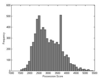
The total area of the pitch is 7140 units and Team A controls a small portion of it around 2500 units. The low ownership is reflected by Team B being in possession of the ball for 78% of the match and Team A playing defensively. Possession scores of 3600 (about half of the pitch) is an effect of the time spent in kickoff position after each goal is scored and is not a representation that Team A had influence on the pitch.
It was also observed that larger team spaces usually correspond to attacking game plays and smaller ones to defensive ones. In terms of spatial configurations, larger team spaces facilitates easier passing and movements to intercept stray balls which helps in build up for attacking game play. In contrast, smaller team spaces indicate tight configurations better suited to protect specific small areas, intercept passes through and shots in that region.
However, from the data recorded it is not conclusive that larger team spaces would mean that a team in on attack alone. The team must also be in possession of the ball.
The relationship between team space and ball position was examined. In the figure below from [19], positive values indicate more control exerted by Team A, and negative values indicate increased control by Team B. The plot of ball x-position has been rescaled in amplitude, but has not been altered frame wise. The x-axis of ball position is defined as the line passing through the center of both goal mouths.

A relationship can be seen between the two plots, with both having similar major features. These features appear in close phase to one another with a difference varying between 20 to 30 frames. This relationship is evident in all of the seven matches.
The experiments indicate that once a team has possession of the ball, it adopts a broad spatial configuration, which facilitates passing and safe movement about the pitch.
Law concluded that better representation of the game is needed and that Voronoi diagrams as a representation technique for control of pitch might be a good idea as a strong correlation between ball movement and distribution of team space was established. It meant that the control a team exerts over the pitch is proportional to its attacking or defending stance.
3.3 Extending Dominant Region to Build Complex Tactics
Nakanishi et al. and used dominant regions in their work to build tactics and strategies for RoboCup Small Sized League [21] [22]. In [21] a method for cooperative play among 3 robots in order to score a goal is presented. Experimental results indicate that the success rate of the play depends strongly on the arrangement of the robots.
One robot kicks the ball and the other receives and shoots the ball with no delay. The technique had a problem as their ball passing skill was slow and a good opponent team would be able to intercept the pass. The challenge is if the first robot kicks the ball faster, it is likely for the receiving robot to miss the ball as its ability is limited by the vision processing and physical movement (locomotion) and therefore, there’s a maximal kicking speed limit enforced for this type of game play to work. There is a need to add more complexity to game play so that the players keep on passing the ball around and avoid the opponent’s defense.
A common strategy in actual soccer is to do a pseudo pass. Player A actually needs to pass the ball to Player B but there is a good chance that the pass would be intercepted, therefore, Player A passes the ball to Player C who immediately kicks the ball to Player B. However, such a game play has a few technical issues when applied to robots:
- Where should three robots position on the field?
- How is the second robot controlled?
The usual way for defense is to approach the opponent possessing the ball, direct play and 1-2-3 shoot play help in avoiding the defense by drawing the opponent’s defenders towards one agent while it passes the ball to someone else. This makes the opponent’s defensive strategy to fail or at least confuse them.
A direct play is where a robot changes the direction of the ball’s velocity without holding or dribbling the ball, but by kicking the ball in a new direction as soon as it arrives. This type of play helps in continuous passing among teammates without stopping the ball’s motion.
A 1-2-3 shoot play is where a robot passes the ball to a teammate who in turn immediately passes it to a third agent.
Let A be a robot holding the ball and B be a cooperating robot.
Step 1: The robot B moves to an open location that has an open shooting line to the goal.
Step 2: The robot A kicks the ball towards the robot B.
Step 3: Measuring the ball speed using vision system, calculate the position and time that the ball meets robot B.
Step 4: The robot B moves to Bt2 meeting at exactly time t2.
Step 5: The proximity sensor of the robot B detects the moment that the ball touches to the robot B and kicks the ball at that moment.

To achieve a 1-2-3 shoot, the teammate robots should have an advantage that a pass is possible between them without being intervened by the opponents. The Dominant Region Method provides the framework for necessary computations for this advantageous scenario.
The dominant region is a variant of voronoi diagram. It is calculated based on two agents only, one of which is a teammate and the other is the opponent. It simply divides the pitch into two areas, one where the teammate can reach faster and the other where opponent can reach faster.
Let and be an initial velocity and an acceleration of the teammate robot, and and be those of the opponent. Let and be the current positions of the teammate and opponent robot, respectively. Then, for given position , the distance between each robot and the given position and arrival time are given by the following:
![]()
Solving the above equations with respect to and , respectively, we obtain:

The dominant region can be generalized to multiple teammates and opponents but it would make the computations too complex as we’ll need to perform the computations for each pair of teammate and opponent.

Using the positions of teammates it is easy to infer the dominant regions. From the figure on the left (taken from [21]), it can be seen that teammate B has an open line of attack to than teammate A.
However, if teammate A tries to pass the ball to teammate B it will be very easy to intercept for the opponents.
If there are three teammates, the risk of getting the ball intercepted would be reduced as shown in the figure below (taken from [21]).

However, simple collaborations are still easier to predict and therefore, the opponents have chances to intercept the ball.
The algorithm to select 1-2-3 Shoot strategy is simple to compute and incorporates conditions where an agent first checks if it has a clear line of shot, if not, then open space is searched and another teammate reaches that position. If the second player doesn’t have a clear line to shoot, another agent moves in and the three agents then execute the 1-2-3 Shoot strategy.
The algorithm for 1-2-3 Shoot is as follows:
- The robot C moves to the open space that has a shoot line to the goal.
- If the pass line crosses the opponent’s dominant region, the robot B moves to the vertex of the near equilateral triangle. As a result a clear pass line is made in the teammate dominant region. The robot B turns to robot C.
- The robot A kicks the ball to the robot B, then the robot B kicks it to the robot C according to the direct play algorithm.
- The robot C kicks the ball toward the goal mouth.
Nakanishi et al. present two algorithms for computing dominant regions and a tactic to break away from a marking opponent player in [22]. The first algorithm is a rough implementation of approximate Dominant Region Diagram computation as presented by [23]. However, the algorithm required 143 seconds to compute the DR on the specific hardware they were using and therefore, needed some optimization in terms of running time. The second algorithm uses an incremental approach for generating partial DR and returned results in sub-millisecond time.
Using the second algorithm as a basis, Nakanishi presented an algorithm that allowed agents to break away from a marking opponent.
The results and tactics discussed in [21] and [22] are very promising; however, we must consider that these are implemented on Small Sized League where wheeled robots are used instead of biped humanoids. This makes it easy for Small Sized League participants to incorporate such tactics as their locomotion does not need to take care of balance.
3.4 Modeling Strategies and Tactics using Situational Calculus
Dylla et al. attempted to model soccer strategies and tactics in a way that could be used in multiple robotic soccer leagues. They presented their initial work on a top-down model to formalize the soccer theory such that specifications and executions could be possible in [24] and later refined in [25].
Dylla et al. chose [26] as a basis for their source on soccer theory as it presented tactics rather than training. They interpreted soccer strategy as a tuple str = <RD, CBP> where RD is a set of role descriptions that describes the overall required abilities of each player position in relation to CBP and CBP is a set of complex behavior patterns.
For a given strategy str, the associated role description rd ϵ RD can be described by the defense tactics task, the offense tactics task, the tactical abilities and the physical skills. For example, the offensive phase can be structured into four sub-phases: gaining ball possession, building up play, final touch and shooting.
The players are distinguished with three positional roles (back, midfield, forward) and sides (left, center, right). The combination of roles and sides would identify a particular player’s type. The following figure from [24] lays out these roles and sides on a soccer pitch.
Each agent needs to have such a view of the game. As this would give the complete view of the game, it is referred to as world model. The world model is created and shared by all the team mates.
Some predicates are introduced such as hasBall and reachable.
These predicates would help in building up actions such as pass would suppose that the receiver would be able to receive it therefore reachable predicate would help the agent sending the pass to determine if a certain team-mate can reach and receive the pass.

Dylla et al.’s work uses a logic based programming language called Golog (introduced by [27]) that is based on situational calculus. Situational Calculus is a second order language proposed by John McCarthy in 1963. There are three important entities in situational calculus: actions, situations and objects. The world state is characterized by relations and functions with a situation term as their argument.
Later, in [25], Dylla et al. used Readylog which is a variant of Golog as Readylog provided frameworks to work directly with continuous change, concurrency, exogenous and sensing actions, probabilistic projections, decision theoretic planning employing Markov Decision Process.
The first problem when modeling human soccer theory to robotic soccer was modeling spatial relations. For coaching human soccer players, it is natural to convey instructions in fuzzy manner such as ‘when the ball is NEAR do XYZ’ without explicitly defining as to what exactly near is. Dylla et al. used equivalence classes to model distances and angles.
The fundamental predicate reachable needed to be modeled. To express reachability, a model that takes into account the amount of free space is needed. Voronoi Diagram and their dual Delauny Triangulation were used for this purpose. The Voronoi diagram in this particular case gives information about which position is closest to which player.
Using these constructs it is easy to construct and express complex tactics and game plays using second order propositional logic. Dylla et al. present two examples in [25] for counter-attack and build-up play.
3.5 Agent positioning using Voronoi Diagram
Dashti et al. describe a flexible dynamic positioning method on Voronoi Cells in [28]. The method also uses attraction vectors that indicate agent’s tendency to specific objects in the field with respect to the game situation and other agents. They compare their results with a situation based strategic positioning (SBSP) method in RoboCup Soccer Simulation.
SBSP needs definitions for home positions to work and according Dashti et al. this is a major constraint. SBSP uses inputs such as game state, team formation, player’s roles and their current positions to calculate an agent’s target position. The target position is computed as the weighted sum of its home position and current position of the ball as an attraction point.
DPVC calculates attraction vectors, roles and target positions without needing to use formation information. In [28] vector sum of different attraction vectors determine an agent’s movement. This vector is a function of ball position, opponent and team mate goal positions in the field. Attraction vectors also differ for each role and are influenced by game situation.
Since DPVC does not use team formation, there is a chance of crowding and thereby multiple agents converging at a common region therefore, each teammate must repulse each other to ensure that they are spread out. This repulsion is achieved through Voronoi Diagram. Once a Voronoi Diagram for a particular instant is created, the agents are forced to move to the center of gravity of their Voronoi cell.
Although Fortune’s algorithm [10] computes a Voronoi diagram in O(n log(n)) time, it cannot compute just a single Voronoi Cell, and since each agent needs to know about their own Voronoi cell a modified algorithm called CalculateVC is presented that returns the agent’s Voronoi cell only. Although it’s complexity is O(n2) but it is a good enough tradeoff since only one Voronoi cell has to be computed.
The vector that defines the force on the agent towards the center of the Voronoi cell is defined as the Voronoi vector. If an agent is near to the center of its cell, its distance from other agents is near optimal. However, in a real system, the environment is dynamic and changing constantly therefore, attractions are continuously applied to agents and they never get to an equilibrium state, instead they are forced on equivalency paths that are updated continuously.
Adding points for opponents would enable agents to distribute between open spaces and break the opponent’s defenses as well as at the same time avoid getting marked by them. This strategy would also enable the agents to continuously move towards opponent goal.
Applying both attraction vectors as well as Voronoi vectors enables agents to repulse each other and at the same time attract ball or opponent goal. It is suggested that Voronoi vectors are applied with care such that it doesn’t cause abrupt changes in the agent’s direction.
The major advantage of DPVC is that number of agents in a particular role is not fixed and results in lesser predictability in the team’s strategy.
Dashti et al.’s further work in [29] presents comparison between DPVC, SBSP, Dynamic Positioning and Positioning using Machine Learning. It further describes Lloyd’s Method for constructing centroidal Voronoi Diagram.
There are various optimization techniques discussed in [29] for having smoother movements of agents while making them pursue for their Voronoi Cell centers.
Akiyama and Noda use similar methods using Delauny Triangulation instead of Voronoi Diagram in [30]. A comparison with SBSP is made and introduces NGnet, an artificial neural network that uses Normalized Gaussian function rather than the usual sigmoid as the activation function.
The results show that when the ANN was trained using a biased data set that restricted movements of teammates even when one of their teammate had the ball resulted in less goals scored.
3.6 Choosing the Player to Attack/Intercept the Ball
Wu et al. describe a simple strategy that employs Voronoi Diagram for selecting the most suitable player to attack/intercept a moving ball in [31]. The first step is to construct Voronoi Diagram to identify the duty areas for each agent as depicted in the diagram below (taken from [31]).

The diagram depicts a very common scenario where the ball is moving across a number of players. In a greedy approach first agent 1 would try to intercept the ball followed by agent 2, agent 3 and then agent 4. Depending on the ball’s velocity, there is a very high chance that the agents nearest to the ball would not be able to reach it. Using a Voronoi diagram, it would be easy to exclude agent 2 in trying to intercept the ball.
Pairing this up with an estimated ball velocity, it is possible that only one of the agents makes a move towards the ball, while the rest reposition based on the changes in the Voronoi distribution.
3.7 Selecting Tactics based on Markov Decision Process
Once an agent has got the ball, it now has to decide what to do. Guerrero et al. [32] presented an integrated multi-agent decision making framework which addresses the problems of where to kick the ball to, and how to position in the field when the robot is in supporting role (does not have the ball) based on MDP. They have divided their team into three simplistic groups – i) goalie; ii) main player (possessing the ball); and iii) supporting players. Their work concerns with the second and third type only; and specifically to their kicking and positioning decisions. Their model makes considerations for the fact that the agent’s decision must balance defensive and offensive game plays.
There had been work that addressed these issues in isolation – that is the model either focuses on kicking decisions or on positioning decisions. As discussed in Section 3.5, Dashti et al.’s DPVC ([28] and [29]) use Voronoi Diagram whereas Nakanishi et al. use Dominant region in [22] as discussed in Section 3.3 focus on positioning only.
Guerrero et al. suggest the use of a coarse approximated MDP as an MDP although could be computed offline and stored for retrieval during real-time usage would require too much memory making it not a feasible option. The approximation is based on the facts that the reward is based on the position of the ball and that the ball moves faster than the agents who retain their pose for a certain amount of time while the ball does change its position. The result is an MDP that would not be valid for a longer period of time.
The terminal states are the two states where a goal could be scored, either in the team’s own goal or in the opponent’s goal. The ball control policy is divided into two sub-policies and depends on which team is in possession of the ball.
Action decision is made based on the selection of appropriate kick and it angle. The resultant position is calculated based on ideal execution of the action scenario.
Role assignment and positioning are implemented in a similar way as the kicking action. It allows for variable role assignment as well as variable number of attackers and defenders. Since the paper focuses on Standard Platform League, there is one goalie and only 1 or 2 robots are positioning therefore, the positioning agents need to consider only the positions they could reach. In case where the kicking agent is a teammate then it will kick the ball in the area that maximizes the attack reward value. Positioning agent’s best choice in this scenario is to move to the point to be able to reach the kicked ball. This would effectively position the agent in an attacking position.
For the alternate scenario, when the kicking agent is an opponent, then the agent needs to position themselves in such a way so as to minimize the reward value in order to intercept the incoming ball.
The MDP based comprehensive strategy presented in [32] relies heavily on the fact that Standard Platform League has only two available players. It will become too complex to implement on other leagues where the number of teammates are 9- or 11- a side.
4. Final Word
Seven different strategies have been researched and presented in this research survey. All of them are not implementable to 3D Soccer Simulation League, however, a roadmap for implementing some of them can significantly improve the performance of teams in 3D Soccer Simulation League.
5. References
| [1] |
|
| [2] |
|
| [3] | “A* search algorithm,” [Online]. Available: http://en.wikipedia.org/wiki/A*_search_algorithm#Pseudocode. |
| [4] |
|
| [5] |
|
| [6] |
|
| [7] |
|
| [8] |
|
| [9] |
|
| [10] |
|
| [11] |
|
| [12] | “Delaunay triangulation,” [Online]. Available: http://en.wikipedia.org/wiki/Delaunay_triangulation#Relationship_with_the_Voronoi_diagram. |
| [13] |
|
| [14] |
|
| [15] |
|
| [16] |
|
| [17] |
|
| [18] |
|
| [19] |
|
| [20] |
|
| [21] |
|
| [22] |
|
| [23] |
|
| [24] |
|
| [25] |
|
| [26] |
|
| [27] |
|
| [28] |
|
| [29] |
|
| [30] |
|
| [31] |
|
| [32] |
|
